


The paper describes a standardized way to link structure (physical layout) with semantics (meaning). The terminology of rows and columns is claimed to be insufficient to capture the underlying meaning of data being represented in tables. In the Tidy Data perspective, each table represents a type of observational unit, with each variable being a column and each observation a row.
There is this really nice illustration from Hadley’s R for Data Science page that illustrates this organization:
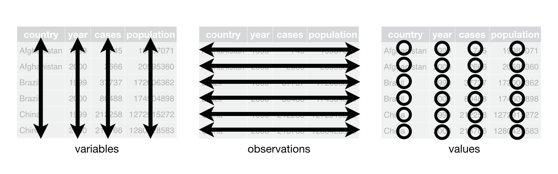
For clarifying the entities involved, the following vocabulary is presented:
- Dataset: This is the higher level organization that describes a collection of values.
- Values: Every value belongs to a variable and an observation. There is a further distinction given with numbers said to be quantitative and strings qualitative.
- Variable: A variable contains all values that measure a particular attribute across units.
- Observation: An observation contains all values measured on the same unit across attributes.
A sample dataset can be represented using this terminology as:
| Variable 1 | Variable 2 | Variable 3 | |
|---|---|---|---|
| Observation 1 | Value 1 | Value 2 | Value 3 |
| Observation 2 | Value 4 | Value 5 | Value 6 |
| Observation 3 | Value 7 | Value 8 | Value 9 |
The author designates this as a canonical standard into which other tables can be transformed. For instance, this table:
| Treatment A | Treatment B | |
|---|---|---|
| John Smith | — | 2 |
| Jane Doe | 16 | 11 |
| Mary Johnson | 3 | 1 |
and its transpose:
| John Smith | Jane Doe | Mary Johnson | |
|---|---|---|---|
| Treatment A | — | 16 | 3 |
| Treatment B | 2 | 11 | 1 |
can be organized in the Tidy Data format as:
| Person | Treatment | Result |
|---|---|---|
| John Smith | a | — |
| Jane Doe | a | 16 |
| Mary Johnson | a | 3 |
| John Smith | b | 2 |
| Jane Doe | b | 11 |
| Mary Johnson | b | 1 |
The original dataset can be thought of as having the following observation/variable structure where pairs are produced from the product:
{ John, Jane, Mary } * { Treatment A , Treatment B }
with each cell of the cross product having a value.
The second is a transpose, which can be represented as:
{ Treatment A, Treatment B } * { John, Jane, Mary }
These are then denormalized to a table with only the following columns:
{ Person, Treatment, Result }
where rows fully capture the data previously structured in cross-tab tables.
The ways in which you can instate these transformations and related ones are given special names in the paper. The process of denormalizing the table is called melting. The converse of this process is termed casting, where you lift the contents of a column as a header. Some tables require melting, and certain others require casting in order to be in the tidy data format.
It is said that the denormalized table tells us more about the structure of the observations. In certain cases, this representation allows for omitting measurements that can't be made, like the count of pregnant males. Nonsensical observations can be cast out of the table when they are put into the tidy data format. My thinking is that there is perhaps no free lunch, and this gain might be offset by some wrinkle appearing in the standard elsewhere.
It is worth remarking that the paper doesn't make the kind of ontology adopted in the background explicit. This presents some difficulty in following the rationale behind choosing a particular transformation in a particular context. A related aspect is that in a given analysis, multiple schematic organizations may be performed by prioritizing certain observations over others, and there is no guideline here on how to settle on a schema. I think both of these concerns might have been addressed with good clarity had the author provided a philosophical discussion about the underlying ontology that motivates these.
In Tidy data, each variable forms a column, each observation a row, and each type of observational unit forms a table. This is said to be Codd’s 3rd normal form with the constraints framed in statistical language. It is claimed that vector programming languages are well suited to tidy data because they ensure that values of different variables from the same observation are always paired.
Fixed vs. Measured Variables
A classification is brought in on variables as fixed / measured. Fixed variables are those that are known in advance and describe the experimental design such as the dates on which an experiment is conducted and readings are taken. Meanwhile, measured variables are those that are actually measured in the study, say, the temperature on a particular day. When constructing a tidy table, fixed variables come first, followed by measured variables.
Messy datasets
Messy data is any arrangement other than the tidy one. Here are a few ways in which datasets can be messy:
- Column headers are values and not variable names
- Multiple variables in one column
- Variables in both rows and columns
- Multiple types of observational units in the same table
- A single observational unit in multiple tables
Example:
The following is an untidy table:
| Religion | Male | Female |
|---|---|---|
| Atheist | 3 | 4 |
| Hindu | 14 | 12 |
| Jew | 3 | 5 |
| Christian | 10 | 9 |
| Islam | 4 | 4 |
| Buddhist | 2 | 4 |
Making it tidy results in the following:
| Religion | Gender | Count |
|---|---|---|
| Atheist | Male | 3 |
| Hindu | Male | 14 |
| Jew | Male | 3 |
| Christian | Male | 10 |
| Islam | Male | 4 |
| Buddhist | Male | 2 |
| Atheist | Female | 4 |
| Hindu | Female | 12 |
| Jew | Female | 5 |
| Christian | Female | 9 |
| Islam | Female | 4 |
| Buddhist | Female | 4 |
There is a certain issue I stumbled on in this paper. It appears on a first reading that there is
inconsistency in the beginning when casting is introduced in 12 b). Here, the tmax and tmin are
cast,
and it is said to be done in order to achieve the observations in a single line, but this kind of
intermixing was said to be problematic in the previous example of religions, and melting was used to make it tidy. This puzzled me for a while.
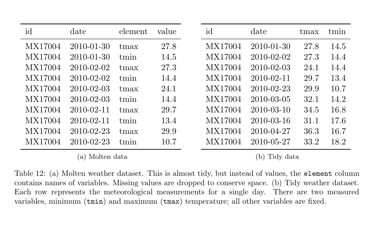
It turns out that the reason for applying these two criteria is not pointed out when introduced in 12 b) but gets addressed in the “Modelling”“ section 4.3. This gets elucidated by contrasting the example of the left / right hands as making Table 14 a) the tidy one, while Table b) is said to be apt for observations over different days. These details were kept implicit in the mind of the author when Table 12 a) and b) were introduced. This caused a certain confusion, which I think could have been avoided by making it explicit early on. Or even better, by supplying the ontological criteria for such transformations which would have made the reading process much smoother.
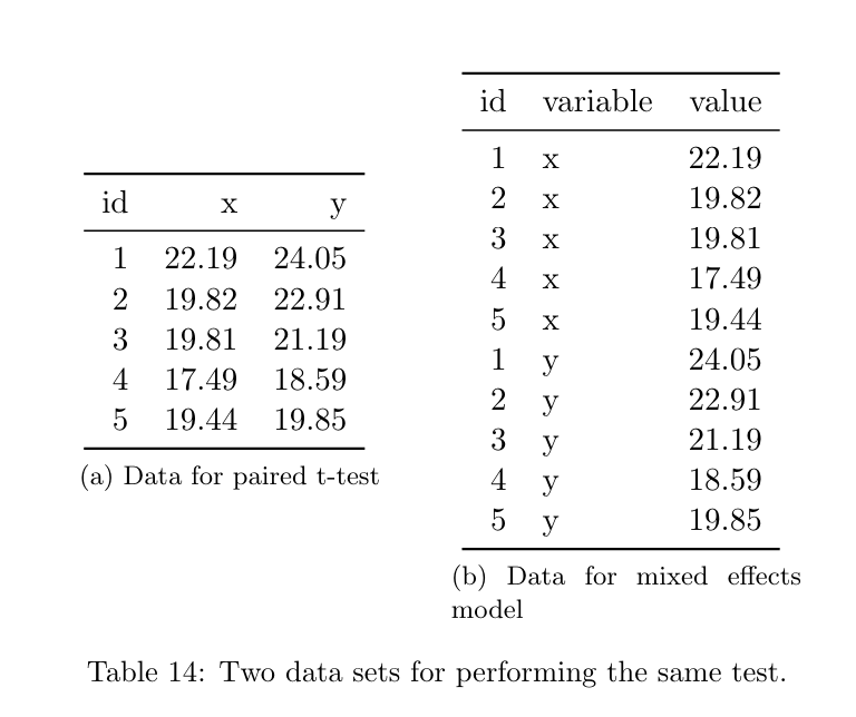
I think the ontology underlying here is that in Table a), a body is seen as the object of observation
with
the left and right arms as the fixed variables, while for the example of weather data in Table b), the observation turns out to be a
day
of the month, making a month the object for grounding. The tmin / tmax per day are to be noted as measured variables, while
id, date, month, etc., are fixed variables. Datasets are to be grouped by the
observational
unit. I could be off with this discussion of
the
underlying ontology, but in any case, making this kind of philosophical assumption implicit doesn’t
help
a first-time reader getting exposed to the idea of Tidy Data to make sense of how to organize these
tables using the transforms outlined.
This is said to be closely related to the idea of database normalization, where each fact is expressed only in one place and as stated before is Codd’s Third Normal Form stated in statistical language.
🔍 To research further: What is the distinction between a t-test and a mixed effects model?